PostgreSQL limit的神奇作用介绍_F11 - 专业站长和开发者的学习网站

网站首页收藏本站

广告位联系

APP正在开发中...

返回顶部

分享到

PostgreSQL limit的神奇作用介绍

数据库其他 来源：互联网作者：佚名发布时间：2022-09-18 19:43:33 人浏览

摘要

最近碰到这样一个SQL引发的性能问题，SQL内容大致如下： 1 2 3 4 5 6 7 SELECT * FROM t1 WHERE id = 999 AND (case $1 WHEN true THEN info = $2 ELSE info = $3 end) limit 1; 开发反应这条SQL加上limit 1之后过了一段时

最近碰到这样一个SQL引发的性能问题，SQL内容大致如下：

SELECT *

FROM t1

WHERE id = 999

AND (case $1

WHEN 'true' THEN

info = $2

ELSE info = $3 end) limit 1;

开发反应这条SQL加上limit 1之后过了一段时间从原先的索引扫描变成了全表扫描，一个简单的limit 1为何会产生这样的影响，我只取一条数据不是应该更快了吗？

下面我们就从这条SQL开始说起。

首先我们先看下这个表结构，比较简单，info列上有个索引，如下所示：

bill=# \d t1

Table "public.t1"

Column | Type | Collation | Nullable | Default

----------+-----------------------------+-----------+----------+---------

id | integer | | |

info | text | | |

crt_time | timestamp without time zone | | |

Indexes:

"idx_t1" btree (info)

并且info列是没有重复值的，这意味着无论where条件中传入什么变量都肯定是能走索引扫描的。那为什么加上limit 1后会变成全表扫描呢？

我们先看看这条SQL之前正常的走索引的执行计划：

QUERY PLAN

------------------------------------------------------------------------------------------------------------------

Limit (cost=0.56..3.18 rows=1 width=45) (actual time=0.027..0.027 rows=0 loops=1)

-> Index Scan using idx_t1 on t1 (cost=0.56..3.18 rows=1 width=45) (actual time=0.025..0.026 rows=0 loops=1)

Index Cond: (info = 'bill'::text)

Filter: (id = 999)

Planning Time: 0.158 ms

Execution Time: 0.057 ms

(6 rows)

而现在的执行计划却是这样的：

Limit (cost=0.00..0.35 rows=1 width=45) (actual time=487.564..487.564 rows=0 loops=1)

-> Seq Scan on t1 (cost=0.00..170895.98 rows=491791 width=45) (actual time=487.562..487.562 rows=0 loops=1)

Filter: ((id = 999) AND CASE $1 WHEN 'true'::text THEN (info = $2) ELSE (info = $3) END)

Rows Removed by Filter: 6000000

Planning Time: 0.119 ms

Execution Time: 487.595 ms

(6 rows)

奇怪的是下面的全表扫描加上limit后cost反而更低，但实际时间竟然长了这么多。而当我们将日志中获取的绑定变量值带入SQL中再去查看执行计划时，仍然是走索引扫描。既然如此，那比较容易想到的就是plan cache导致的执行计划错误了。

由于在PostgreSQL中执行计划缓存只是会话级别的，PostgreSQL在生成执行计划缓存前，会先走5次custom plan，然后记录这5次总的custom plan的cost, 以及custom plan的次数，最后生成通用的generic plan。

以后，每次bind时，会根据缓存的执行计划以及给定的参数值计算一个COST，如果这个COST 小于前面存储的custom plan cost的平均值，则使用当前缓存的执行计划。如果这个COST大于前面存储的custom plan cost的平均值，则使用custom plan(即重新生成执行计划)，同时custom plan的次数加1，custom plan总成本也会累加进去。

既然如此，我们使用prepare语句再测试一次：

bill=# prepare p1 as select * from t1 where id = 999

bill-# and (case $1 when 'true' then info = $2 else info = $3 end) limit 1;

PREPARE

bill=# explain analyze execute p1('true','bill','postgres');

QUERY PLAN

------------------------------------------------------------------------------------------------------------------

Limit (cost=0.56..3.18 rows=1 width=45) (actual time=0.831..0.831 rows=0 loops=1)

-> Index Scan using idx_t1 on t1 (cost=0.56..3.18 rows=1 width=45) (actual time=0.830..0.830 rows=0 loops=1)

Index Cond: (info = 'bill'::text)

Filter: (id = 999)

Planning Time: 0.971 ms

Execution Time: 0.889 ms

(6 rows)

bill=# explain analyze execute p1('true','bill','postgres');

QUERY PLAN

------------------------------------------------------------------------------------------------------------------

Limit (cost=0.56..3.18 rows=1 width=45) (actual time=0.038..0.039 rows=0 loops=1)

-> Index Scan using idx_t1 on t1 (cost=0.56..3.18 rows=1 width=45) (actual time=0.037..0.037 rows=0 loops=1)

Index Cond: (info = 'bill'::text)

Filter: (id = 999)

Planning Time: 0.240 ms

Execution Time: 0.088 ms

(6 rows)

bill=# explain analyze execute p1('true','bill','postgres');

QUERY PLAN

------------------------------------------------------------------------------------------------------------------

Limit (cost=0.56..3.18 rows=1 width=45) (actual time=0.036..0.036 rows=0 loops=1)

-> Index Scan using idx_t1 on t1 (cost=0.56..3.18 rows=1 width=45) (actual time=0.035..0.035 rows=0 loops=1)

Index Cond: (info = 'bill'::text)

Filter: (id = 999)

Planning Time: 0.136 ms

Execution Time: 0.076 ms

(6 rows)

bill=# explain analyze execute p1('true','bill','postgres');

QUERY PLAN

------------------------------------------------------------------------------------------------------------------

Limit (cost=0.56..3.18 rows=1 width=45) (actual time=0.051..0.051 rows=0 loops=1)

-> Index Scan using idx_t1 on t1 (cost=0.56..3.18 rows=1 width=45) (actual time=0.049..0.050 rows=0 loops=1)

Index Cond: (info = 'bill'::text)

Filter: (id = 999)

Planning Time: 0.165 ms

Execution Time: 0.091 ms

(6 rows)

bill=# explain analyze execute p1('true','bill','postgres');

QUERY PLAN

------------------------------------------------------------------------------------------------------------------

Limit (cost=0.56..3.18 rows=1 width=45) (actual time=0.027..0.027 rows=0 loops=1)

-> Index Scan using idx_t1 on t1 (cost=0.56..3.18 rows=1 width=45) (actual time=0.025..0.026 rows=0 loops=1)

Index Cond: (info = 'bill'::text)

Filter: (id = 999)

Planning Time: 0.158 ms

Execution Time: 0.057 ms

(6 rows)

bill=# explain analyze execute p1('true','bill','postgres');

QUERY PLAN

-----------------------------------------------------------------------------------------------------------------

Limit (cost=0.00..0.35 rows=1 width=45) (actual time=487.564..487.564 rows=0 loops=1)

-> Seq Scan on t1 (cost=0.00..170895.98 rows=491791 width=45) (actual time=487.562..487.562 rows=0 loops=1)

Filter: ((id = 999) AND CASE $1 WHEN 'true'::text THEN (info = $2) ELSE (info = $3) END)

Rows Removed by Filter: 6000000

Planning Time: 0.119 ms

Execution Time: 487.595 ms

(6 rows)

果然在第6次时出现了我们想要的结果！

可以看到前5次索引扫描的cost都是3.18，而全表扫描的cost却是0.35，所以自然优化器选择了全表扫描，可为什么cost变低了反而时间更久了呢？解答这个问题前我们先要来了解下limit子句的cost是如何计算的。

limit cost计算方法：

先从一个最简单的例子看起：

我们只取1条记录，cost很低，时间也很少。

bill=# explain analyze select * from t1 limit 1;

QUERY PLAN

--------------------------------------------------------------------------------------------------------------

Limit (cost=0.00..0.02 rows=1 width=45) (actual time=0.105..0.106 rows=1 loops=1)

-> Seq Scan on t1 (cost=0.00..110921.49 rows=5997449 width=45) (actual time=0.103..0.103 rows=1 loops=1)

Planning Time: 0.117 ms

Execution Time: 0.133 ms

(4 rows)

加上where条件试试呢？

cost一下子变成3703.39了，似乎也很好理解，因为我们在进行limit前要使用where条件进行一次数据过滤，所以cost变得很高了。

bill=# explain analyze select * from t1 where id = 1000 limit 1;

QUERY PLAN

---------------------------------------------------------------------------------------------------------

Limit (cost=0.00..3703.39 rows=1 width=45) (actual time=0.482..0.483 rows=1 loops=1)

-> Seq Scan on t1 (cost=0.00..125915.11 rows=34 width=45) (actual time=0.480..0.481 rows=1 loops=1)

Filter: (id = 1000)

Rows Removed by Filter: 1008

Planning Time: 0.117 ms

Execution Time: 0.523 ms

(6 rows)

但当我们换个条件时结果又不同了：

从where id=1000变成 id=999，cost竟然一下子又降低到0.13了，似乎找到了前面全表扫描的limit cost比索引扫描还低的原因了。

bill=# explain analyze select * from t1 where id = 999 limit 1;

QUERY PLAN

-------------------------------------------------------------------------------------------------------------

Limit (cost=0.00..0.13 rows=1 width=45) (actual time=0.041..0.042 rows=1 loops=1)

-> Seq Scan on t1 (cost=0.00..125915.11 rows=983582 width=45) (actual time=0.040..0.040 rows=1 loops=1)

Filter: (id = 999)

Rows Removed by Filter: 107

Planning Time: 0.114 ms

Execution Time: 0.079 ms

(6 rows)

那么这个limit的cost究竟是如何计算的呢，为什么条件不同cost能差这么多呢？

下面给出limit cost计算方法：

limit_cost = ( N / B ) * A

N：表示limit取的数据，如limit 1则N=1；

B：表示估算得到的总记录数；

A：表示估算的总成本。

例如上面cost=0.13的执行计划中，N = 1，B = 983582，A = 125915.11，那么limit cost便是：

(1/983582)*125915.11 = 0.128，即执行计划中显示的0.13。

简而言之就是如果通过where条件筛选得到的行数越多，那么limit cost就会越低。

知道了这些我们再回过头去看那条SQL就清楚了，因为where id = 999这个条件的数据比较多，这也就导致了即使是全表扫描limit cost也很低，甚至比索引扫描还低。

SELECT *

FROM t1

WHERE id = 999

AND (case $1

WHEN 'true' THEN

info = $2

ELSE info = $3 end) limit 1;

但是需要注意的是，我们即使使用explain analyze看到的执行计划中的cost也是一个估算值，并不是实际值，尽管这个和实际值差距不会很大，但如果cost本身就很小，那么还是会带来一点误解的。

例如前面的SQL我想要提高全表扫描的limit cost让其大于索引扫描，这样优化器便会一直选择索引扫描了，于是我将limit 1改成limit 100（即增加N的值），但是却仍然没有起作用：

QUERY PLAN

------------------------------------------------------------------------------------------------------------------------------------------------------

Limit (cost=0.56..5.58 rows=1 width=53) (actual time=0.049..0.051 rows=1 loops=1)

-> Index Scan using idx_scm_bind_scm_customer_id_index on scm_bind t (cost=0.56..5.58 rows=1 width=53) (actual time=0.049..0.050 rows=1 loops=1)

Index Cond: ((scm_customer_id)::text = 'wmGAgeDQAAXcpcw9QWkDOUQsIDI1xOqQ'::text)

Filter: ((bind_status)::text = '2'::text)

Planning Time: 0.160 ms

Execution Time: 0.072 ms

(6 rows)

Time: 0.470 ms

QUERY PLAN

---------------------------------------------------------------------------------------------------------------------------------------------------------------------------------

Limit (cost=0.00..8.90 rows=100 width=53) (actual time=1047.859..16654.360 rows=1 loops=1)

-> Seq Scan on scm_bind t (cost=0.00..552392.00 rows=6208050 width=53) (actual time=1047.858..16654.357 rows=1 loops=1)

Filter: (((bind_status)::text = '2'::text) AND CASE $1 WHEN 'client'::text THEN ((scm_customer_id)::text = ($2)::text) ELSE ((scm_customer_id)::text = ($3)::text) END)

Rows Removed by Filter: 12169268

Planning Time: 0.147 ms

Execution Time: 16654.459 ms

(6 rows)

Time: 16654.924 ms (00:16.655)

下面的全表扫描是第6次传入参数得到的，可以看到全表扫描的cost是8.9，而索引扫描是5.58，那应该不会选择cost更高的8.9啊？

而当我们去跟踪实际的cost就可以发现：

$1 = {magic = 195726186, raw_parse_tree = 0x15df470,

query_string = 0x16d65b8 "PREPARE p1(varchar,varchar,varchar) as\n select\n t.scm_sale_customer_id,\n t.scm_customer_id\n from\n scm_bind t\n where t.bind_status = '2'\n and (case $1 when 'client' then scm_customer_id ="..., commandTag = 0x95b5ba "SELECT", param_types = 0x16d66c8, num_params = 3, parserSetup = 0x0, parserSetupArg = 0x0, cursor_options = 256, fixed_result = true,

resultDesc = 0x16d66e8, context = 0x15df250, query_list = 0x16dbe80, relationOids = 0x16e6138, invalItems = 0x0, search_path = 0x16e6168, query_context = 0x16dbd70, rewriteRoleId = 10,

rewriteRowSecurity = true, dependsOnRLS = false, gplan = 0x16ff668, is_oneshot = false, is_complete = true, is_saved = true, is_valid = true, generation = 6, next_saved = 0x0,

generic_cost = 8.8979953447539888, total_custom_cost = 52.899999999999999, num_custom_plans = 5}

实际索引扫描的cost大约数10.58，和执行计划中显示的还是有一定差距的。

让我们言归正传，既然知道了为什么全表扫描的limit cost更低，我们再来解决下一个问题：为什么cost很低但实际执行时间却这么长？

让我们再看看执行计划：

Limit (cost=0.00..0.35 rows=1 width=45) (actual time=487.564..487.564 rows=0 loops=1)

-> Seq Scan on t1 (cost=0.00..170895.98 rows=491791 width=45) (actual time=487.562..487.562 rows=0 loops=1)

Filter: ((id = 999) AND CASE $1 WHEN 'true'::text THEN (info = $2) ELSE (info = $3) END)

Rows Removed by Filter: 6000000

Planning Time: 0.119 ms

Execution Time: 487.595 ms

(6 rows)

仔细观察可以发现，原先应该作为索引的info列的过滤条件，竟然整个作为了filter条件去进行数据过滤了。

那么最后的问题就出现在这个where条件中的case when表达式了，因为在case when表达式进行过滤前，绑定变量还没有传入实际的值，而优化器对于不确定的值自然无法选择是否去走索引了，这里不得不吐槽一下这种写法。。。

因此对于优化器计算limit cost时，只知道where id = 999会得到大量的数据，而无法判断后面的case when里面会得到多少数据，因此虽然后面的条件只会得到很少一部分数据，但是优化器生成limit cost时估算得到的总记录数B只是根据id = 999去判断，导致估算的cost很低，但实际却只得到很少的数据，要去表中过滤大量数据。

不得不感叹这个“简单”的SQL竟然包含着这么多知识。

您可能感兴趣的文章 :

原文链接 : https://foucus.blog.csdn.net/article/details/122107557

Tag : PostgreSQL(22)limit(8)

六大主流数据同步工具对比：DataX、Airbyte、Cana

当数据量变大、数据源复杂、实时需求提高，很多团队在选数据同步工具时犯难。本文对 DataX、Airbyte、Canal、Debezium、Fivetran 与 Apache SeaTun
解读SQL生成工具

SQL 生成工具可用于测试Parser与其他数据库产品的兼容性，通过解析YACC语法文件中的产生式，生成对应的SQL语句，再使用数据库执行该SQL，根
SQLite3在嵌入式C环境中存储音频/视频文件的最优

SQLite3 在嵌入式C环境中存储音频/视频文件的专业方案在嵌入式系统中存储大型媒体文件需要平衡存储效率、访问速度和资源限制。以下是针
嵌入式数据库SQLite 3配置使用

0、惨痛教训随着管理开发的项目体积越来越庞大，产品系统涉及的数据量也越来越多，并且伴随着项目不久就要交付给甲方了。如果项目的
Sqlite3基本语句及安装过程

SQLite3简介 SQLite3是一款轻量级的、基于文件的开源关系型数据库引擎，由 D. Richard Hipp 于 2000 年首次发布。它遵循 SQL 标准，但与传统的数据
在SQLite中进行批量操作的有效实现方法

SQLite 是一个轻量级的关系型数据库管理系统，因其高效性和易用性而广受欢迎。在许多应用场景中，批量操作的需求是不可避免的，例如在
一文介绍在Hive中NULL的理解

在 Hive 中，NULL 是一个特殊的值，表示未知或缺失。任何与NULL的比较操作（如=,,,=,=,）都会返回NULL，而不是TRUE或FALSE。 1.NULL 的比较规则在
Navicat Premium 12数据库管理解决方案

Navicat Premium 12是一款全面的数据库管理工具，支持多种数据库系统如MySQL、MariaDB、Oracle、SQL Server、PostgreSQL等。它提供了多数据库连接、数据
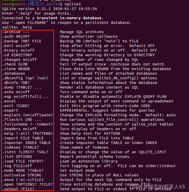
sqlite3命令行工具使用介绍

一、启动与退出启动数据库连接 1 2 3 sqlite3 [database_file] # 打开/创建数据库文件（如 test.db） sqlite3 # 启动临时内存数据库 (:memory:) sqlite3 :m
StarRocks简介与搭建使用介绍

StarRocks简介 StarRocks 是一款高速、实时、全场景的MPP（大规模并行处理）分析型数据库系统，专为现代数据分析场景设计，强调亚秒级查询性